Imputation concordance tables

This page explains the imputation concordance tables that are produced during most runs of IMPUTE2.

Home

What is a concordance table? (top)

Every run of IMPUTE2 produces a concordance table, except under certain settings that are not commonly used. A concordance table shows the results of an internal cross-validation that the program performs automatically. For this analysis, IMPUTE2 masks the genotypes of one variant at a time in the study data (Panel 2), then imputes the masked genotypes with information from the reference data and nearby study variants. The imputed genotypes are then compared with the original genotypes to evaluate the quality of the imputation. The results are summarized in a table like the one below:

Concordance table

If you are interested in the results of this experiment at a given variant, you can find this information in the _info file printed by IMPUTE2. The concord_typeX column shows the concordance between input genotypes and best-guess imputed genotypes at each variant, while the r2_typeX column gives the squared correlation between input genotypes and expected genotypes (or "dosages") from imputation. Note that the cross-validation cannot be performed at variants that were not provided in a Panel 2 input file (-g or -known_haps_g), so reference-only variants are assigned values of -1 in the _info file. To learn more about the format of this output file, see here.

How are concordance tables made? (top)

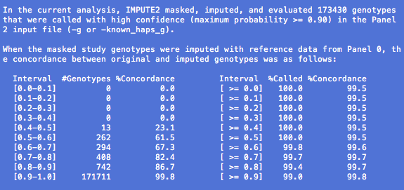
Only variants with input data from a -g or -known_haps_g file are masked and imputed in this analysis. When a -known_haps_g file is provided, all input genotypes are treated as being true. When a -g file is provided, we make hard genotype calls by applying a threshold (default = 0.9) to the maximum value in each input probability triple. For example, a genotype with P(G=0,1,2) = (0.03, 0.95, 0.02) would be called as a '1' (heterozygous), while a genotype with P(G=0,1,2) = (0.1, 0.7, 0.2) would be left uncalled and omitted from the concordance calculations.

The genotype probabilities from imputation are used somewhat differently. In the first three columns of the table, we assign each imputed genotype to a bin (Interval) based on its maximum posterior probability. Then, for each bin we report the number of imputed genotypes that passed the calling threshold in the input data (#Genotypes). We then convert the imputed probabilities to 'best-guess' genotypes: for each posterior probability triple, we select the genotype with the highest value, regardless of magnitude. Finally, we compare the input genotype calls with the best-guess imputed genotypes and report the concordance (%Concordance) within each bin.

In the last three columns of the table, we again bin the imputed genotypes based on their maximum posterior probabilities, but this time the binning is cumulative: the bin at the bottom of the table includes only genotypes that were confidently imputed (max prob >= 0.9), while each bin above includes all genotypes that pass a more lenient certainty threshold. These thresholds are shown in the fourth column (Interval). The fifth column (%Called) shows the percentage of imputed genotypes that pass a given probability threshold, where the denominator is the total number of imputed genotypes for which hard calls are available in the input data. The sixth column (%Concordance) shows the percentage of imputed genotypes in a given bin that match the masked input genotypes.

What can I do with a concordance table? (top)

We can learn a couple of things from this kind of analysis. First, the results can alert us to problems in the imputation: if the concordance between imputed and input genotypes is abnormally low, it may indicate that something went wrong in the analysis or input files. A useful summary statistic is the number in the upper righthand corner of the table, which gives the overall concordance from the cross-validation. This number should typically be around 95%; it may be lower in certain populations or regions of the genome, but if it is much lower then you may need to double-check the analysis. If you are worried about your results, please feel free to contact us. If you do, please send a _summary output file from IMPUTE2.

Concordance tables can also be used to predict the general quality of imputed genotypes at SNPs where we do not know the true genotypes. SNPs on GWAS microarrays tend to be easier to impute than untyped SNPs of the same frequency, so the cross-validation results may be somewhat optimistic, but they are often useful for relative comparisons -- say, between different parameter settings of IMPUTE2.

Finally, the per-variant results of the cross-validation in the output _info file can help identify poorly genotyped SNPs and strand flips. For example, an input SNP that has a low concord_typeX value (implying that the imputed genotypes do not agree with the original genotypes) and a high info_typeX value (implying that the imputation is confident) might be worth investigating or removing from subsequent imputation runs.

Multiple reference panels (top)

If you provide two reference panels to IMPUTE2, the program will perform the cross-validation in two different ways. First it will use only a single reference panel (Panel 0) to mimic Type 0 SNPs, and then it will use both reference panels together (Panels 0 and 1) to mimic Type 1 SNPs. In this case, IMPUTE2 will print two concordance tables -- one for each type of reference SNP. Note that the same masked study genotypes are used to evaluate accuracy in both cases; the only difference is how much reference data we allow the program to see when imputing the masked genotypes.

Where can I find the concordance table? (top)

The concordance table is printed at the end of an IMPUTE2 run. One copy is printed to STDOUT, and another copy is printed in the _summary output file.