GENECLUSTER
Updates:- 01/04/2011, new plot.signal.r supplied with executables
- 04/05/2011, Zhan Su will be leaving his academic post from 08/05/2011, after which only minimal support for this software will be provided. He can be contacted on zhan dot su dot work at gmail dot com.
GENECLUSTER is a novel program for
detecting association in genome-wide case-control studies based on a
set of known haplotypes (like the HapMap Phase II haplotypes). The
program is designed to work seamlessly with the output of the genotype
calling program CHIAMO
and the simulation program HAPGEN,
and the input of the association analysis program SNPTEST.
|
 |
Overview (top)
GENECLUSTER detects association between SNP genotype data and case-control status by constructing an approximate genealogy for the case-control (study) sample. Briefly, at each site of interest GENECLUSTER searches through the branches in the constructed genealogy for evidence of a causal mutation. This approach offers several avdantages to the traditional SNP-based approach (where single SNPs are independently tested for association), they include the ability to:- detect association with SNPs not typed in the study sample, like imputation, and also with SNPs that are not typed in the reference panel, which imputation can not;
- detect allelic heterogeneity (the presence of two or more causal muations in linkage disequilibrium), where it exists;
- provide a significant boost in signal for association under allelic heterogeneity;
- identify the causal SNPs in a region of association; and
- estimate the effect sizes in a region of association.
GENECLUSTER is applicable to genotype data with missing data. It requires similar compuational resources as IMPUTE.
Contributors (top)
The following people have contributed to the development of the methodology and software for GENECLUSTERZhan Su, Niall Cardin, Peter Donnelly and Jonathan Marchini
Input files (top)
GENECLUSTER requires the same input files as IMPUTE and in the same format. Other than the case and control genotype files (GENECLUSTER accepts more than one case or control genotype file), the following resources are required:- reference panel of phased haplotypes and legend file
- fine-scale recombination rates
- strand file (if applicable)
In addition GENECLUSTER also needs a set of trees constructed for the reference panel at the set of positions where association is tested. You can download the trees and the other resource files (with HapMap haplotypes as the reference panel) here. If you would like to use your own reference panel haplotypes or build trees at a custom set of positions then a custom tree building program is available upon request.
Running GENECLUSTER (top)
GENECLUSTER must be run in two stages- GC2 must to be executed on all case and control genotype files individually, but with the same tree, reference haplotype, legend and recombination rates files. The GC2 output files for each case and control sample should then be passed onto GC3 to analyse for association. More details on running GC2 are given below.
- GC3 uses the output files from GC2 to produce output files that summarises the evidence for association and allelic heterogeneity. More details on running GC3 are given below
Example
An example data set is included with the excutables for download, in the folder example. The example folder folder contains- data for two control cohorts: example/controls1.gen and example/controls2.gen
- data for one case cohort: example/cases.gen
- strand file: example/strand.txt
- recombination rates file: example/genetic_map.txt
- haplotype reference panel file: example/panel.txt
- legend file for the haplotype reference panel: example/legend.txt
- a tree file: example/tree_file.txt
| ./GC2 -h ./example/panel.txt -l ./example/legend.txt -g ./example/controls1.gen -m ./example/genetic_map.txt -int 38640000 39110000 -tree_file ./example/tree_file.txt -strand ./example/strand.txt -o ./example/controls1.gc2.txt.gz |
| ./GC2 -h ./example/panel.txt -l ./example/legend.txt -g ./example/controls2.gen -m ./example/genetic_map.txt -int 38640000 39110000 -tree_file ./example/tree_file.txt -strand ./example/strand.txt -o ./example/controls2.gc2.txt.gz |
| ./GC2 -h ./example/panel.txt -l ./example/legend.txt -g ./example/cases.gen -m ./example/genetic_map.txt -int 38640000 39110000 -tree_file ./example/tree_file.txt -strand ./example/strand.txt -o ./example/cases.gc2.txt.gz |
GC2 will write the intermdiate files into the folder ./example/GC2_files and once it completes you should run GC3:
| ./GC3 -int 38640000 39110000 -tree_file example/tree_file.txt -o example/ex.gs -mutation_models 1.0 1.0 0.0 -controls ./example/controls1.gc2.txt.gz ./example/controls2.gc2.txt.gz -cases ./example/cases.gc2.txt.gz |
Running GC2 (top)
GC2 is a command line program. This program constructs an approximate genealogy for each study sample based on the genealogy for a haplotype reference panel at every location within an interval of interest, specified by the -int flag, where a tree for the reference panel is available. GC2 should be run on all case and control samples first and their output files should then be passed onto GC3 to test for association.IMPORTANT:
- It is very important that the SNP data used by GC2 are clean, i.e. low missing data rate, high call confidence etc. As a guideline, for the WTCCC2 study, we filtered out all SNPs with a minor allele frequency less than 0.001, or information measure (see SNPTEST webpage for more details) less than 0.975, or HWE pvalue less than 1e-20, or missing data rate of more than 0.02. You can either remove any bad SNPs directly from the genotype data files, or use the -exclude_snps flag to GC2 to remove them from the analysis.
- The set of SNPs used by GC2 MUST be the same for the controls and cases data. This means that any SNPs excluded from the cases data must also be excluded from the control data and vice versa. Note that the -exclude_snps flag accepts multiple files.
- The reference panel must be well matched to the study data in terms of ethnicity. In order to maximise power, the study data and reference panel should also have a large number of SNPs in common. If the reference panels supplied below are not well matched to your study, then you can phase a subset of your controls data and use them as the reference panel (we recommend a panel size of around 200 haplotypes), and build trees using Niall Cardin's TREESIM software.
| Flags |
Required/Optional |
Default | Description |
| -g
<file> |
Required | File containing a set of
genotypes for the set if individuals. The file format is described in
detail on the FILE
FORMAT WEBPAGE. The file format is the same as the output
format from our genotype calling program CHIAMO.
NOTE 1 : The SNPs MUST appear in base-pair position order (lowest to highest) i.e. the 3rd column of this file must be sorted. NOTE 2 : Base-pair positions of SNPs must use the same genome build as that used in the haplotype file. NOTE 3 : GC2 supports gzipped files but they must have the extension .gz. |
|
|
-h <file> |
Required |
|
File containing a set of known
haplotypes for the region of interest. The alleles of the haplotypes
should be coded as 0 and 1. The format of this input file is one line
per SNP and one column per haplotype. |
| -o
<file> |
Required | The GC2 output file, which
contain details of the pseudo-genealogies for the study sample based on
the reference panel haplotypes. The file should then be passed onto GC3
as input. GC2 output files can be quite big and we recommend that you
name the output files with a ".gz" extension so that they will
automatically be gzipped by GC2. |
|
|
-int <lower> <upper> |
Required |
|
Lower are Upper boudaries (in base pair position) of the region in which tests of association are to be carried out. Only positions for which a tree is available will be analysed. |
|
-l <file> |
Required | |
Legend file for haplotypes file
which give rs ID, position and the alleles that are coded as 0 and 1 in
the haplotypes file. The alleles should be taken from A, C, G and T.
Note that this file needs a header line (see the example file
legend.txt for details) |
|
-m <file> |
Required | |
Fine-scale recombination map covering the region at which analysis is required. There is one line for each position on the map. The first column contains the base pair position, the 2nd column contains the recombination rate in cM/Mb to the next point on the map and the 3rd column contains the recombination map position in cM.Note that this file needs a header line (see the example file map.txt for details) |
|
-tree_file <file> |
Required | |
A file containing a set of trees for the reference panel haplotypes at locations where an association test is to be performed. Trees for the HapMap haplotypes are available for download at the bottom of this page. All gzipped files must have a ".gz" extension. |
|
-Ne <int> |
Optional | 11418 | Sets effective population size that scales the fine-scale recombination map for the given population. For example, -Ne 11000 sets the effective population size to 11000. For autosomal chromosomes, we highly recommend the values 11418 for CEPH, 17469 for Yoruban and 14269 for Chinese Japanese populations. |
|
-buffer <int> |
Optional |
500 |
To avoid edge effects, the program includes genotypes either side of the interval specified by the the -int flag. This option specifies the length of the buffer region (in kb) at each end of the interval. |
|
-call_thresh <double> |
Optional |
0.9 |
Threshold for calling genotypes
in genotype input file. The genotype with the maximum probability will
be used if that probability is above the threshold. Otherwise the
genotype will treated as missing. |
| -exclude_snps <file> | Optional | Exclude a set of genotyped SNPs
(i.e. SNPs that occur in the file specified by the -g option) with ID
equal to those listed in the file. The IDs can be either the rs ID or
the alternate ID given in the first column of the genotype file. These
SNPs will not be used for analysis. |
|
| -exclude_samples <file> | Optional | Exclude a list of individuals
from the analysis. The IDs in the file should be the ID that appears in
the first or second column of the sample file. A sample file number be
provided using the -sample flag. |
|
| -sample |
Optional |
Sample file (see FILE FORMAT WEBPAGE for more details) containing the unique identifiers for each individual in the genotype file. Is only used when the -exclude_samples flag is used. | |
| -strand
<file> |
Optional | File listing the strand
orientation of the SNPs in the genotype file relative to the
orientation of the alleles in the haplotypes file. This is file is
required if the orientation of alleles at SNPs in the haplotype and
genotype files does not match up. The file should contain a line for
each SNP in the genotype file with two entries (i) the base-position of
the SNPs, and (b) the strand (+ or -) of the alleles in the genotype
file. SNPs do not have to be in the same order as in the
genotypes file and the file can include SNPs that are not in the
genotypes file i.e. if the genotypes file has had some SNPs filtered
out. Take a look at the example files for an illustration of the
required format. NOTE : It is critical that the alleles used to code genotypes in the haplotype file and the genotype file match up. If not, then the quality of imputation may decrease substantially. Great care should be taken in constructing a strand file for your data. |
Running GC3 (top)
GC3 is a command line program. It performs tests of association based on the GC2-constructed genealogies for the case and control samples. The disease model assumes one or more causal mutations occurred in the genealogy of the case-control sample. We consider up to three different disease models: 1-mutation model, 2-mutation model and 3-mutation model, which assumes 1, 2 or 3 causal mutations occurred in the genealogy. The evidence for each disease model is compared to the evidence for the null model (where no causal mutation occurred in the genealogy), and is summarised by a Bayes factor.| Flags | Required/Optional | Default | Description |
|
-controls <file1> <file2> ... |
Required |
|
The set of GC2 output files produced for each control sample. You must run GC2 on all case and control genotype files (with the same tree, haplotype reference, legend and recombination rates files) before running GC3. |
| -cases <file1> <file2>... | Required | |
The set of GC2 output files produced for each case sample. You must run GC2 on all case and control genotype files (with the same tree, haplotype reference, legend and recombination rates files) before running GC3. |
|
-int <lower> <upper> |
Required |
|
Lower and upper boudaries (in base pair position) of the region in which tests of association are to be carried out. Only positions for which a tree is available will be analysed. |
|
-modelA <prior1> <prior2> <prior3> |
Optional |
0.5 0.5 0 | The prior weights on the
1-mutation, 2-mutation and 3-mutation models. Only models with prior
weight greater 0 are implemented, so by default the 3-mutation model,
which is computationally intensive, will not be implemented. The prior
weights determine the Bayes factor for association under all of the
implemented mutation models in the output file. See below for more details. NOTE 1 :It is not important to specify the specific values of the prior, only that the models that you intend to run have prior weight greater than 0. NOTE 2 :It is not important that the prior weights add to 1, GC3 will normalise them to a prior probability distribution. |
|
-ntree <n> |
Optional |
1 | The maximum number of trees to use for analysis (if a tree file contains more than n trees). |
|
-o <file> |
Required | |
The file where the results should be written to. There will also be a file with .aux concatanated to the filename, which contains a copy of the command line summary output. |
|
-tree_file <file> |
Required | The same tree file that was provided to GC2. | |
|
-rprior <a> <b> |
Optional | See right column |
The parameters of the beta(a,b) penetrance prior. If not specified then will be set to a = p*50 and b = (1-p)*50, where p is the proportion of controls your total sample. |
Analysing GENECLUSTER output (top)
GENECLUSTER summarises the evidence for association in terms of a Bayes factor. The Bayes factor (BF) is the factor by which the prior odds for association should be adjusted conditional on the case-control data, i.e. posterior odds = prior odds * BF (for more details on Bayes factors see Balding, D. (2006)). One of the advantages of using Bayes factor is that there is no need to be adjusted for multiple testing; a Bayes factor threshold for significance should reflect the prior odds of association. For example, a threshold of 10^4 is used on the assumption that there are 1,000,000 independent regions in the genome and 100 of these is involved with disease. The threshold should be adjusted according to the context of the study, for example a lower threshold might be used in a candidate region, to reflect a higher a priori probability of association.An example GENECLUSTER results file has the following columns
- location - the physical location where tests of association have been performed
- ntree - the number of trees used to perform tests of association
- ncontrols - the number of control individuals considered at each location
- ncases - the number of case individuals considered at each location
- alpha - the first parameter of the beta prior on penetrance used for inference
- beta - the second parameter of the beta prior on penetrance used for inference
- mut1 - the Bayes factor under the 1-mutation model of association, 0 if not implemented (see the -modelA option of GC3 for details)
- mut2 - the Bayes factor under the 2-mutation model of association, 0 if not implemented (see the -modelA option of GC3 for details)
- mut3 - the Bayes factor under the 3-mutation model of association, 0 if not implemented (see the -modelA option of GC3 for details)
- mean_mut - the Bayes factor under under the 1-mutation, 2-mutations and 3-mutation models of association, based on the prior on all three models (specified by the -modelA option of GC3)
| location ntree ncontrols ncases alpha beta mut1 mut2 mut3 mean_mut |
| 38640000 1 30 20 2 3 0.6673980344 0.4651869063 0 0.5662924704 |
| 38645000 1 30 20 2 3 0.733595907 0.5241572532 0 0.6288765801 |
| ... |
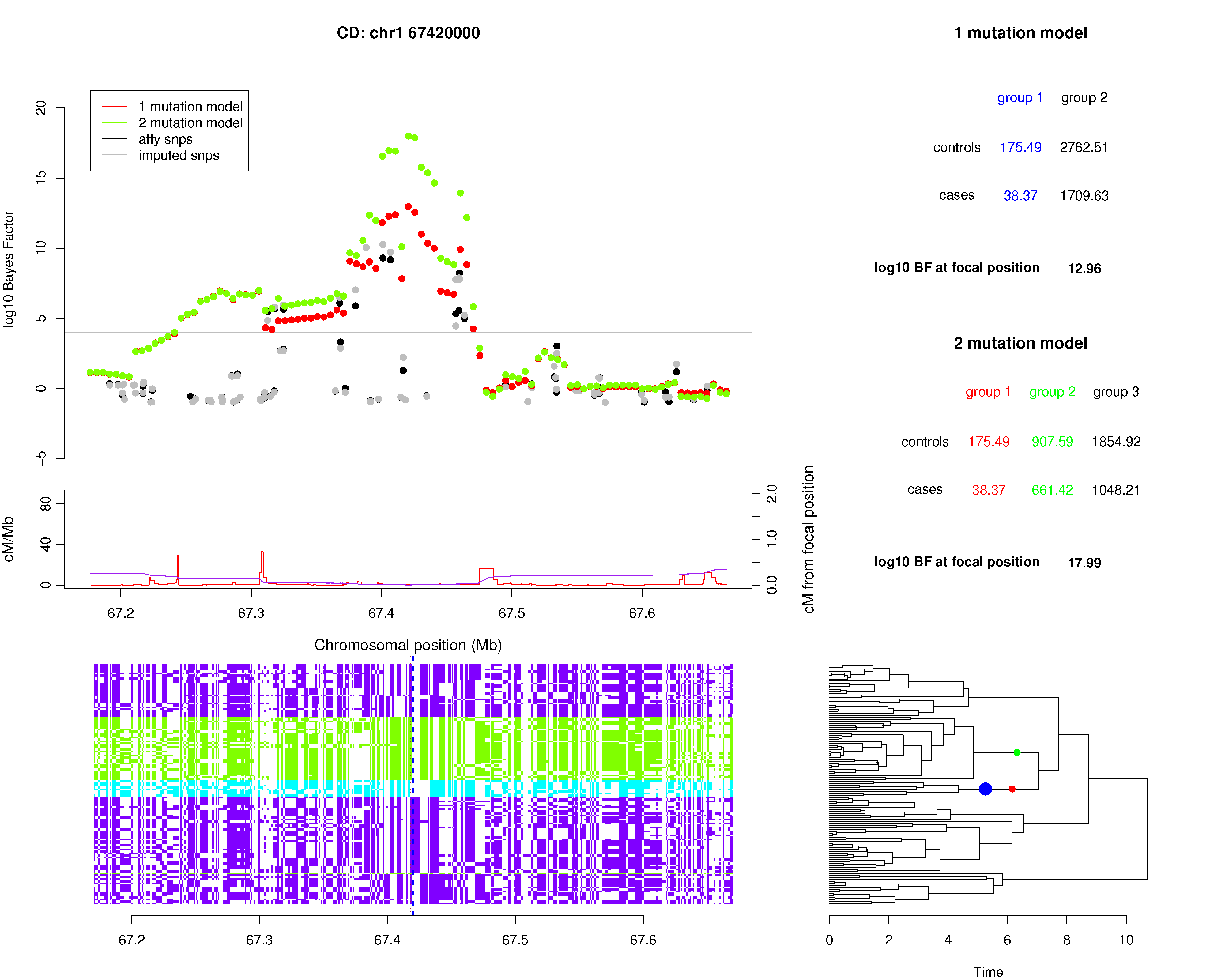
Plotting GENECLUSTER results
To allow better visualisation of the signal across a region of interest, we have provided an R script with the executables, called plot.signal.r, that can:- plot the BFs of the 1-mutation, 2-mutation and 3-mutation models within a specified region, along with BFs produced by other methods if available
- plot the tree of the reference haplotypes at a specified "focal" position within the region
- label on the tree the location of the most likely single causal mutation (under the 1-mutation model) and the most likely pair of causal mutations (under the 2-mutation model)
- a table of relative risk estimates for each of the mutations on the tree
To produce signal plots, you must open R in the GENECLUSTER directory (which contains the GC2 and GC3 executables and the plot.signal.r script) and load the source function and then run the function make.plot. For example, to plot the results of the GC3 output on the example files:
| source("plot.signal.r") |
| make.plot( | gc.file
= "./example/ex.gs", control.gc2.files = c("./example/controls1.gc2.txt.gz", "./example/controls2.gc2.txt.gz"), case.gc2.files = "./example/cases.gc2.txt.gz", legend.file = "./example/legend.txt", log.file = "./example/plot.signal.log", max.location = 39110000, min.location = 38640000, panel.file = "./example/panel.txt", plot.title = "Example signal plot", rates.file = "./example/genetic_map.txt", rs.ids = c("rs2708479", "rs1388587"), tree.file = "./example/tree_file.txt") |
When the rs.ids option is used, the command line output will list the alleles at SNPs with specified rsids (in this example rs2708479 and rs1388587) carried by each reference panel haplotype, in the order that they are plotted (so the first haplotype is at the top of the plot and the last is at the bottom). The command line output will also list the SNPs in the haplotype reference panel that are highly correlated with any of the best fitting mutations labelled on the tree.
Below are details of the options that make.plot takes:
| Flags |
Required/Optional |
Default | Description |
| gc.file |
Required | The GC3 results output file.
Requires the same input value that was provided to the -o
flag for GC3. |
|
| control.gens.files |
Required | A vector of control GC2 output
files. Requires the same input values that were provided to the -controls
flag for GC3. |
|
| case.gens.files |
Required | A vector of case GC2 output
files. Requires the same input values that were provided to the -cases
flag for GC3. |
|
| panel.file |
Required | The reference haplotype file
that was provided to the -h
flag for GC3. |
|
| legend.file |
Required | The legend file, for the
reference haplotypes, that was provided to the -l
flag for GC2. |
|
| rates.file |
Required | The recombination rates file
that was provided to the -r
flag for GC2. |
|
| tree.file |
Required | The tree file, for the reference
haplotypes, that was provided to the -tree_file
flag for GC3. |
|
| min.location |
Required | The physical location of the
left-hand boundary of the region of interest to be plotted. |
|
| max.location |
Required | The physical location of the
right-hand boundary of the region to be plotted. |
|
| focal.posn |
Optional | The focal position of the signal
plot. The right hand side of the signal plot will display the tree and
details of the best fitting mutations at the focal position. If none is
specified then the focal position will be the position with the largest
2-mutation BF. |
|
| log.file |
Optional | A file with the screen output
summary |
|
| plot.title |
Optional | Title of the plot. |
|
| rs.ids |
Optional | A vector of rsids defines a set
of SNPs in the reference panel haplotypes. These SNPs define a set of
haplotype backgrounds in the haplotype reference panel, and panel
haplotype will be coloured according to its background in the left
plot. |
Comparing 1-mutation model against 2-mutation model
The relative values of the Bayes factors for the 1-mutation and 2-mutation provide an indication for the presence of allelic heterogeneity. To calculate the posterior probability of the 2-mutation model, it is given byPr(2-mutation) = BF2/(BF2+BF1) * (Prior2/Prior1),
where BF2 and BF1 are the Bayes factors for 2-mutation and 1-mutation models and Prior2 and Prior1 are the prior probabilities for those two models. For example, if (BF2/BF1)=9 and we assume that both models are equally likely (Prior2 = Prior1), then the posterior probability of the 2-mutation model (i.e. two causal variants in the constructed genealogy) is 0.9. Experience from the WTCCC, WTCCC+ and WTCCC2 projects indicate that there is indeed multiple independent causal SNPs when BF2/BF1 > 10, although there are also examples where the ratio is smaller. (NOTE: You can also compare the 3-mutation model against the 1-mutation model or 2-mutation model this way)
Sometimes the mutations the GENECLUSTER identifies is highly correlated with SNPs in the reference panel. SNPs with r2>0.8 and they will be displayed in the screen output summary. If no SNPs are found for a particular mutation of interest then you might still be able to manually find a set of SNPs that tag the set of haplotypes falling under the mutation.
Download (top)
HAPGEN2 is available free to use for academic use only. Please see the LICENCE here and also included with the package.Pre-compiled versions of the program and example files can be downloaded from the links below. We've supplied both static and dynamic versions of the Linux executables. If you intend to run GENECLUSTER on a machine running an old kernel then you probably want to use the dynamic version. If you have any problems getting the program to work on your machine please contact me.
| Platform |
File |
| Linux
(x86_64) Static Executable |
genecluster_r84_x86_64.tgz |
| Mac
OS X Intel |
genecluster_r84_macosx_intel.tgz |
Please fill out the registration form to receive emails about updates to this software
To unpack the files use a command like
| tar zxvf GC_vX.X.X_i386.tgz |
This will create
- executables called GC2 and GC3
- a R script, plot.signal.r, for plotting the tree and best fitting mutations at a choosen position, and
- a directory /example that contains the example files.
Running GENECLUSTER Using with the HapMap Data (top)
A main use of this program will be analysing genotypes based on the HapMap Phase II haplotypes. To facilitate this use we have prepared the HapMap Phase II haplotypes in the format required by GENECLUSTER for all 22 autosomes. Be careful to make sure your genotype data uses base-pair positions that are matched to the genome-build used by the haplotype, rate and strand files. We recommend that genome-wide imputation of genotypes be carried in relatively small chunks to avoid running out of RAM on your computer. For analysis of the WTCCC dataset we used a chunk size of 10Mb. The result files were then concatenated together to produce a single results file for each chromosome. The chunk size can be specifed using the -int option. The-buffer should also be used to avoid edge effects of imputing in relatively small chunks.HapMap rel#24 - NCBI Build 36 (dbSNP b126)
|
Polymorphic files - these files contain SNPs polymorphic in each
panel respectively i.e. the CEU haplotypes only contain data at SNPs that are polymorphic in the CEU panel. The files contain the haplotypes and associated legend files. |
[CEU] [YRI] |
| Recombination
rate files (nb. these are the same as the rel#22 rates) |
[CEU] [YRI] [COMBINED] |
| Strand files | Affy500k
[These
were constructed using these Affymetrix annotation files - Nsp
Sty]
Affy6.0 [These files were created using this Affymetrix annotation file - LINK] |
| Tree files - these files contain the data for marginal trees, constructed under a coalescent model, at locations 1kb apart genome-wide. There is one file for each autosomal chromosome and you must extract the file for the appropriate chromosome before analysis. The program, TREESIM, that constructed these trees can be downloaded from Niall Cardin's webpage. | [CEU] [YRI] |
FAQ (top)
References (top)
Z. Su, N. Cardin, WTCCC, P. Donnelly, J. Marchini (2009) A Bayesian method for detecting and characterizing allelic heterogeneity and boosting signals in genome-wide association studies. Statistical Science, 24(4):430-450. DOI: 10.1214/09-STS311Cardin, N. J. and McVean, G. A. T. (under preparation) Genealogical inference under the coalescent with recombination and the Sequentially Markov Coalescent.
Strange, A., Capon, F., Spencer, C.C.A., Knight, J., (...), Trembath, R.C. (2010) A genome-wide association study identifies new psoriasis susceptibility loci and an interaction between HLA-C and ERAP1. Nature Genetics, 42:985-990.
Chris C.A. Spencer, Vincent Plagnol, Amy Strange, (...), Nicholas W. Wood (2011) Dissection of the genetics of Parkinson's disease identifies an additional association 5' of SNCA and multiple associated haplotypes at 17q21. Hum Mol Genet., 20(2): 345-353.